Hopf Torus (1/3): the equatorial case

In this series of three articles, we will show how to construct Hopf tori.

Hopf tori take their origins in the Hopf map \(S^3 \to S^2\) defined by \[ H(p) = \begin{pmatrix} 2(p_2 p_4 - p_1 p_3) \\ 2(p_1 p_4 + p_2 p_3) \\ p_1^2 + p_2^2 - p_3^2 - p_4^2 \\ \end{pmatrix}. \]

Obviously, this map is not bijective. Its main property is that it sends each great circle of \(S^3\) to a same point of \(S^2\). Thus, it has, say a “pseudo-inverse” \(H^{-1} \colon S^2 \times S^1 \to S^3\) defined by \[ H^{-1}(q,t) = \frac{1}{\sqrt{2(1+q_3)}} \begin{pmatrix} q_1 \cos t + q_2 \sin t \\ \sin t (1+q_3) \\ \cos t (1+q_3) \\ q_1 \sin t - q_2 \cos t \\ \end{pmatrix}. \]

Now let’s introduce the stereographic projection: \[ Stereo \colon S^3 -> \mathbb{R}^3 \\ Stereo \, x = \frac{1}{1-x_4}(x_1, x_2, x_3). \]

Then, we can draw a circle in \(\mathbb{R}^3\) as follows:

• take a point \(q\) on \(S^2\);

• calculate the great circle on \(S^3\) by applying \(H^{-1}(q, S^1)\);

• maps this great circle to \(\mathbb{R}^3\) with the stereographic projection.

In this article, we will show what happens when we take for \(q\) a point on the equator on \(S^2\). Below are the necessary R functions.

hopfinverse <- function(q, t){ 
  1/sqrt(2*(1+q[3])) * c(q[1]*cos(t)+q[2]*sin(t),
                         sin(t)*(1+q[3]),
                         cos(t)*(1+q[3]),
                         q[1]*sin(t)-q[2]*cos(t)) 
}
stereog <- function(x){
  c(x[1], x[2], x[3])/(1-x[4])
}

This is the sphere with the equator:

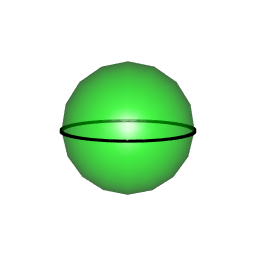
Each point of the equator is mapped to a circle, and the circles form a torus:

library(rgl)
view3d(45,45)
t_ <- seq(0, 2*pi, len=200)
phi <- 0
theta_ <- seq(0, 2*pi, len=300)
for(theta in theta_){
  circle4d <- sapply(t_, function(t){
    hopfinverse(c(cos(theta)*cos(phi), sin(theta)*cos(phi), sin(phi)), t)
  })
  circle3d <- t(apply(circle4d, 2, stereog))
  shade3d(cylinder3d(circle3d, radius=0.1), color="purple")
}

Indeed, we get a torus, made of circles: