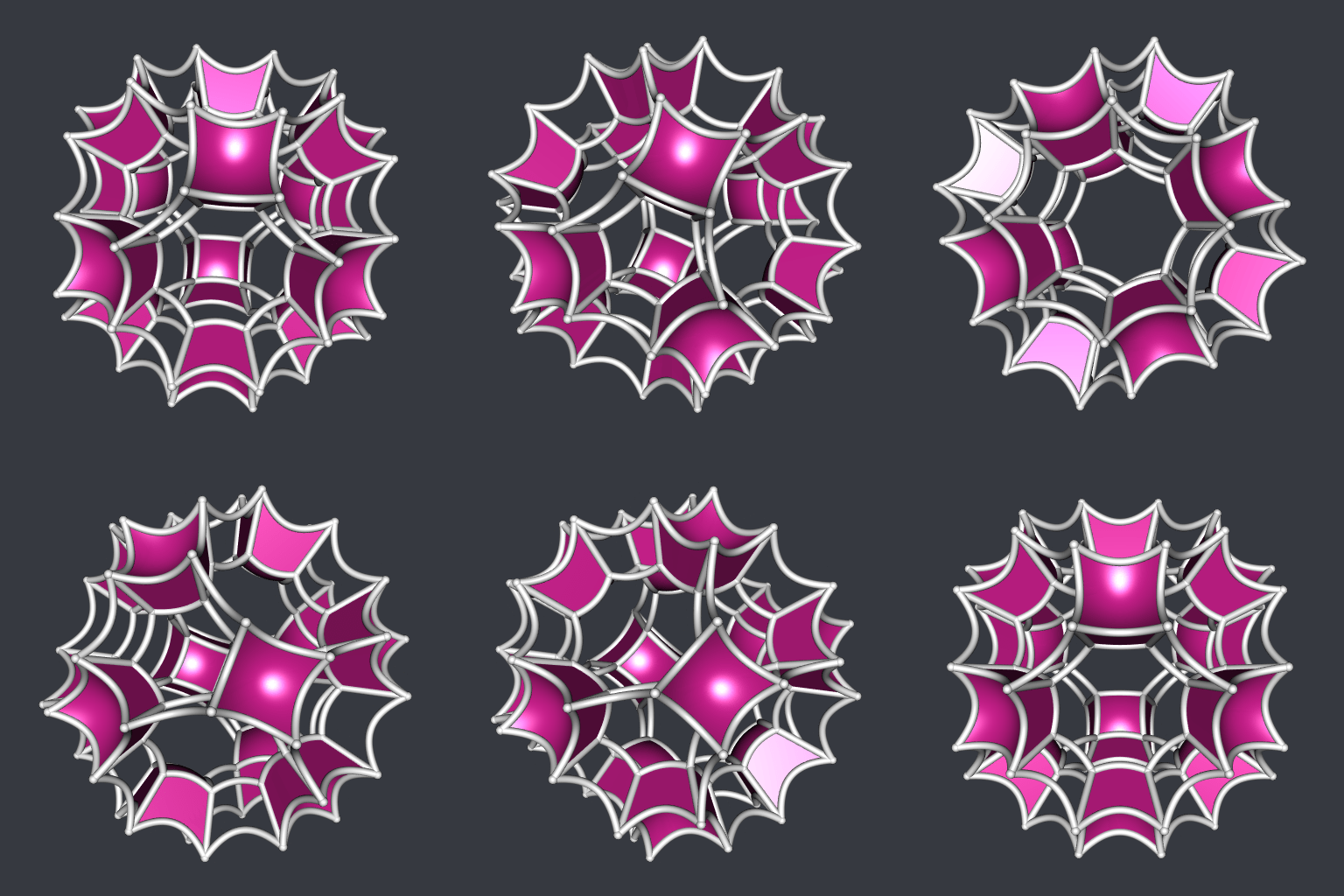
Hyperbolic gircope - using 'cxhull' and 'gyro'
This post is a demonstration of the cxhull and gyro packages. I will use these packages (and others) to draw an hyperbolic version of the stereographic projection of a convex 4D polytope, the gircope or great rhombicuboctahedral prism. The gircope has twenty-eight cells, but I will only draw the twelve cubes among them.
As said in this wiki, the vertices of the gircope are given by all permutations of the first three coordinates of: \[ \left(\pm\frac{1+2\sqrt{2}}{2}, \pm\frac{1+\sqrt{2}}{2}, \pm\frac{1}{2}, \pm\frac{1}{2}\right). \]
I define these vertices in R as follows:
library(gyro)         # to use the `changesOfSign` function
library(arrangements) # to use the `permutations` function
x <- c(
  (1 + 2*sqrt(2)) / 2,
  (1 + sqrt(2)) / 2,
  1/2
)
vertices <- changesOfSign(
  cbind(
    t(apply(permutations(3L), 1L, function(perm) x[perm])),
    1/2
  )
)
Obviously, the vertices of the gircope lie on a sphere centered at the origin:
apply(vertices, 1L, crossprod)
##  [1] 5.62132 5.62132 5.62132 5.62132 5.62132 5.62132 5.62132 5.62132 5.62132
## [10] 5.62132 5.62132 5.62132 5.62132 5.62132 5.62132 5.62132 5.62132 5.62132
## [19] 5.62132 5.62132 5.62132 5.62132 5.62132 5.62132 5.62132 5.62132 5.62132
## [28] 5.62132 5.62132 5.62132 5.62132 5.62132 5.62132 5.62132 5.62132 5.62132
## [37] 5.62132 5.62132 5.62132 5.62132 5.62132 5.62132 5.62132 5.62132 5.62132
## [46] 5.62132 5.62132 5.62132 5.62132 5.62132 5.62132 5.62132 5.62132 5.62132
## [55] 5.62132 5.62132 5.62132 5.62132 5.62132 5.62132 5.62132 5.62132 5.62132
## [64] 5.62132 5.62132 5.62132 5.62132 5.62132 5.62132 5.62132 5.62132 5.62132
## [73] 5.62132 5.62132 5.62132 5.62132 5.62132 5.62132 5.62132 5.62132 5.62132
## [82] 5.62132 5.62132 5.62132 5.62132 5.62132 5.62132 5.62132 5.62132 5.62132
## [91] 5.62132 5.62132 5.62132 5.62132 5.62132 5.62132
We will need the value of the radius of this sphere later, for the stereographic projection:
R <- sqrt(c(crossprod(vertices[1L, ])))The gircope is convex, hence it equals its convex hull. But we have only its vertices so far, and we need its edges, its cells, and its ridges (faces of the cells). This is why we use cxhull now:
library(cxhull)
hull <- cxhull(vertices)
edges <- hull[["edges"]]
cells <- hull[["facets"]]
ridges <- hull[["ridges"]]
A cube has eight vertices, and among the cells of the gircope, only the cubic ones have eight vertices. So we get all the cubic cells like this:
cubicCells <-
  Filter(function(cell) length(cell[["vertices"]]) == 8L, cells)
No we need the faces of the cubes (squares). We can easily get the indices of their vertices but we have to order them. That’s what the polygonize function below does:
polygonize <- function(edges){
  nedges <- nrow(edges)
  indices <- edges[1L, ]
  i <- indices[2L]
  edges <- edges[-1L, ]
  for(. in 1L:(nedges-2L)){
    j <- which(apply(edges, 1L, function(e) i %in% e))
    i <- edges[j, ][which(edges[j, ] != i)]
    indices <- c(indices, i)
    edges <- edges[-j, ]
  }
  indices
}
Now we can get the indices of the vertices of the squares:
squares <- t(vapply(
  do.call(c, lapply(cubicCells, `[[`, "ridges")),
  function(r) polygonize(ridges[[r]][["edges"]]),
  integer(4L)
))
Now, let’s project the 4D vertices to the 3D space, with a stereographic projection:
verts3D <- t(apply(vertices, 1L, function(v){
  v[1L:3L] / (R - v[4L])
}))
We are ready for plotting. We can’t directly draw hyperbolic squares with the gyro package. It only allows to draw hyperbolic triangles, with the gyrotriangle function. So we draw an hyperbolic square by splitting it into two triangles, we merge these two triangles with Morpho::mergeMeshes and we remove the duplicated vertices of the resulting mesh with Rvcg::vcgClean.
library(rgl)
library(Morpho) # to use the `mergeMeshes` function
library(Rvcg)   # to use the `vcgClean` function
s <- 0.5 # hyperbolic curvature
open3d(windowRect = c(50, 50, 562, 562), zoom = 0.8)
bg3d(rgb(54, 57, 64, maxColorValue = 255))
for(i in 1L:nrow(squares)){
  square <- squares[i, ]
  mesh1 <- gyrotriangle(
    verts3D[square[1L], ], verts3D[square[2L], ], verts3D[square[3L], ],
    s = s
  )
  mesh2 <- gyrotriangle(
    verts3D[square[1L], ], verts3D[square[3L], ], verts3D[square[4L], ],
    s = s
  )
  mesh <- vcgClean(mergeMeshes(mesh1, mesh2), sel = c(0, 7), silent = TRUE)
  shade3d(mesh, color = "violetred")
}
for(i in 1L:nrow(edges)){
  edge <- edges[i, ]
  A <- verts3D[edge[1L], ]; B <- verts3D[edge[2L], ]
  tube <- gyrotube(A, B, s = s, radius = 0.025)
  shade3d(tube, color = "whitesmoke")
}
spheres3d(verts3D, radius = 0.03, color = "whitesmoke")
To make the animation, I used the following code.
movie3d(
  spin3d(axis = c(1, 1, 0), rpm = 10),
  duration = 6, fps = 10,
  movie = "pic", dir = ".",
  convert = FALSE,
  startTime = 1/10,
  webshot = FALSE)
This code produces the files pic001.png, … pic060.png. Then I assembled them into a GIF with gifski (you can use ImageMagick instead).


