An example of the Minkowski addition

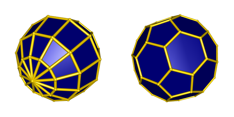
Posted on June 11, 2022 by Stéphane Laurent

Tags: geometry, R, rgl, graphics, C++, Rcpp

Now the MeshesOperations package can construct the Minkowski sum of two polyhedra, thanks to the C++ library CGAL and the R package RcppCGAL. Let’s see an example: the Minkowski sum of Leonardo da Vinci’s 72-sided sphere and a truncated icosahedron. Here are these two polyhedra:

The mesh of the truncated icosahedron is provided by the MeshesOperations package. Here are the (rounded) vertices and the faces of da Vinci’s 72-sided sphere:

vertices <- rbind(
  c( 1.61352, -0.43234,  1.18620),
  c( 1.18118, -1.18118,  1.18620),
  c( 0.43234, -1.61352,  1.18620),
  c(-0.43234, -1.61352,  1.18620),
  c(-1.18118, -1.18118,  1.18620),
  c(-1.61352, -0.43234,  1.18620),
  c(-1.61352,  0.43234,  1.18620),
  c(-1.18118,  1.18118,  1.18620),
  c(-0.43234,  1.61352,  1.18620),
  c( 0.43234,  1.61352,  1.18620),
  c( 1.18118,  1.18118,  1.18620),
  c( 1.61352,  0.43234,  1.18620),
  c( 1.61352, -0.43234, -1.18620),
  c( 1.61352,  0.43234, -1.18620),
  c( 1.18118,  1.18118, -1.18620),
  c( 0.43234,  1.61352, -1.18620),
  c(-0.43234,  1.61352, -1.18620),
  c(-1.18118,  1.18118, -1.18620),
  c(-1.61352,  0.43234, -1.18620),
  c(-1.61352, -0.43234, -1.18620),
  c(-1.18118, -1.18118, -1.18620),
  c(-0.43234, -1.61352, -1.18620),
  c( 0.43234, -1.61352, -1.18620),
  c( 1.18118, -1.18118, -1.18620),
  c( 2.01020,  0.53863,  0.00000),
  c( 1.47157,  1.47157,  0.00000),
  c( 0.53863,  2.01020,  0.00000),
  c(-0.53863,  2.01020,  0.00000),
  c(-1.47157,  1.47157,  0.00000),
  c(-2.01020,  0.53863,  0.00000),
  c(-2.01020, -0.53863,  0.00000),
  c(-1.47157, -1.47157,  0.00000),
  c(-0.53863, -2.01020,  0.00000),
  c( 0.53863, -2.01020,  0.00000),
  c( 1.47157, -1.47157,  0.00000),
  c( 2.01020, -0.53863,  0.00000),
  c( 0.89068,  0.23866,  1.77777),
  c( 0.89068, -0.23866,  1.77777),
  c( 0.65202, -0.65202,  1.77777),
  c( 0.23866, -0.89068,  1.77777),
  c(-0.23866, -0.89068,  1.77777),
  c(-0.65202, -0.65202,  1.77777),
  c(-0.89068, -0.23866,  1.77777),
  c(-0.89068,  0.23866,  1.77777),
  c(-0.65202,  0.65202,  1.77777),
  c(-0.23866,  0.89068,  1.77777),
  c( 0.23866,  0.89068,  1.77777),
  c( 0.65202,  0.65202,  1.77777),
  c( 0.65202, -0.65202, -1.77777),
  c( 0.89068, -0.23866, -1.77777),
  c( 0.89068,  0.23866, -1.77777),
  c( 0.65202,  0.65202, -1.77777),
  c( 0.23866,  0.89068, -1.77777),
  c(-0.23866,  0.89068, -1.77777),
  c(-0.65202,  0.65202, -1.77777),
  c(-0.89068,  0.23866, -1.77777),
  c(-0.89068, -0.23866, -1.77777),
  c(-0.65202, -0.65202, -1.77777),
  c(-0.23866, -0.89068, -1.77777),
  c( 0.23866, -0.89068, -1.77777),
  c( 0.00000,  0.00000,  2.04922),
  c( 0.00000,  0.00000, -2.04922)
)

triangles <- lapply(list(
  c(36, 60, 47), 
  c(37, 60, 36), 
  c(38, 60, 37), 
  c(39, 60, 38), 
  c(40, 60, 39), 
  c(41, 60, 40), 
  c(42, 60, 41), 
  c(43, 60, 42), 
  c(44, 60, 43), 
  c(45, 60, 44), 
  c(46, 60, 45), 
  c(47, 60, 46), 
  c(48, 61, 59), 
  c(49, 61, 48), 
  c(50, 61, 49), 
  c(51, 61, 50), 
  c(52, 61, 51), 
  c(53, 61, 52), 
  c(54, 61, 53), 
  c(55, 61, 54), 
  c(56, 61, 55), 
  c(57, 61, 56), 
  c(58, 61, 57), 
  c(59, 61, 58)
), function(x) x + 1)
quads <- lapply(list(
  c( 0, 11, 24, 35), 
  c(10, 25, 24, 11), 
  c( 9, 26, 25, 10), 
  c( 8, 27, 26,  9), 
  c( 7, 28, 27,  8), 
  c( 6, 29, 28,  7), 
  c( 5, 30, 29,  6), 
  c( 4, 31, 30,  5), 
  c( 3, 32, 31,  4), 
  c( 2, 33, 32,  3), 
  c( 1, 34, 33,  2), 
  c( 0, 35, 34,  1), 
  c(12, 35, 24, 13), 
  c(13, 24, 25, 14), 
  c(14, 25, 26, 15), 
  c(15, 26, 27, 16), 
  c(16, 27, 28, 17), 
  c(17, 28, 29, 18), 
  c(18, 29, 30, 19), 
  c(19, 30, 31, 20), 
  c(20, 31, 32, 21), 
  c(21, 32, 33, 22), 
  c(22, 33, 34, 23), 
  c(12, 23, 34, 35), 
  c( 0, 37, 36, 11), 
  c( 0,  1, 38, 37), 
  c( 1,  2, 39, 38), 
  c( 2,  3, 40, 39), 
  c( 3,  4, 41, 40), 
  c( 4,  5, 42, 41), 
  c( 5,  6, 43, 42), 
  c( 6,  7, 44, 43), 
  c( 7,  8, 45, 44), 
  c( 8,  9, 46, 45), 
  c( 9, 10, 47, 46), 
  c(10, 11, 36, 47), 
  c(12, 49, 48, 23), 
  c(12, 13, 50, 49), 
  c(13, 14, 51, 50), 
  c(14, 15, 52, 51), 
  c(15, 16, 53, 52), 
  c(16, 17, 54, 53), 
  c(17, 18, 55, 54), 
  c(18, 19, 56, 55), 
  c(19, 20, 57, 56), 
  c(20, 21, 58, 57), 
  c(21, 22, 59, 58), 
  c(22, 23, 48, 59)
), function(x) x + 1)
faces <- c(triangles, quads)

Leonardo <- list(vertices = vertices, faces = faces)

In order to produce the above plot with rgl, I triangulated the two meshes. Actually this is not necessary for the Leonardo mesh, since rgl allows meshes with triangles and quads. This is necessary for the mesh of the truncated icosahedron, because it has some faces with more than four sides.

To triangulate a mesh with MeshesOperations, I recommend to use the option numbersType = "lazyExact":

library(MeshesOperations)
tLeonardo <- Mesh(
  mesh = Leonardo, triangulate = TRUE,
  numbersType = "lazyExact"
)
tmesh     <- Mesh(
  mesh = truncatedIcosahedron, triangulate = TRUE,
  numbersType = "lazyExact"
)

Now, here is the code which generates the picture shown before:

library(rgl)
open3d(windowRect = c(50, 50, 850, 450))
mfrow3d(1L, 2L)
view3d(30, 30, zoom = 0.7)
shade3d(toRGL(tLeonardo), color = "navy")
plotEdges(
  tLeonardo[["vertices"]], tLeonardo[["exteriorEdges"]], 
  color = "gold", tubesRadius = 0.06, spheresRadius = 0.08
)
next3d()
view3d(30, 30, zoom = 0.7)
shade3d(toRGL(tmesh), color = "navy")
plotEdges(
  tmesh[["vertices"]], tmesh[["exteriorEdges"]], 
  color = "gold", tubesRadius = 0.06, spheresRadius = 0.08
)

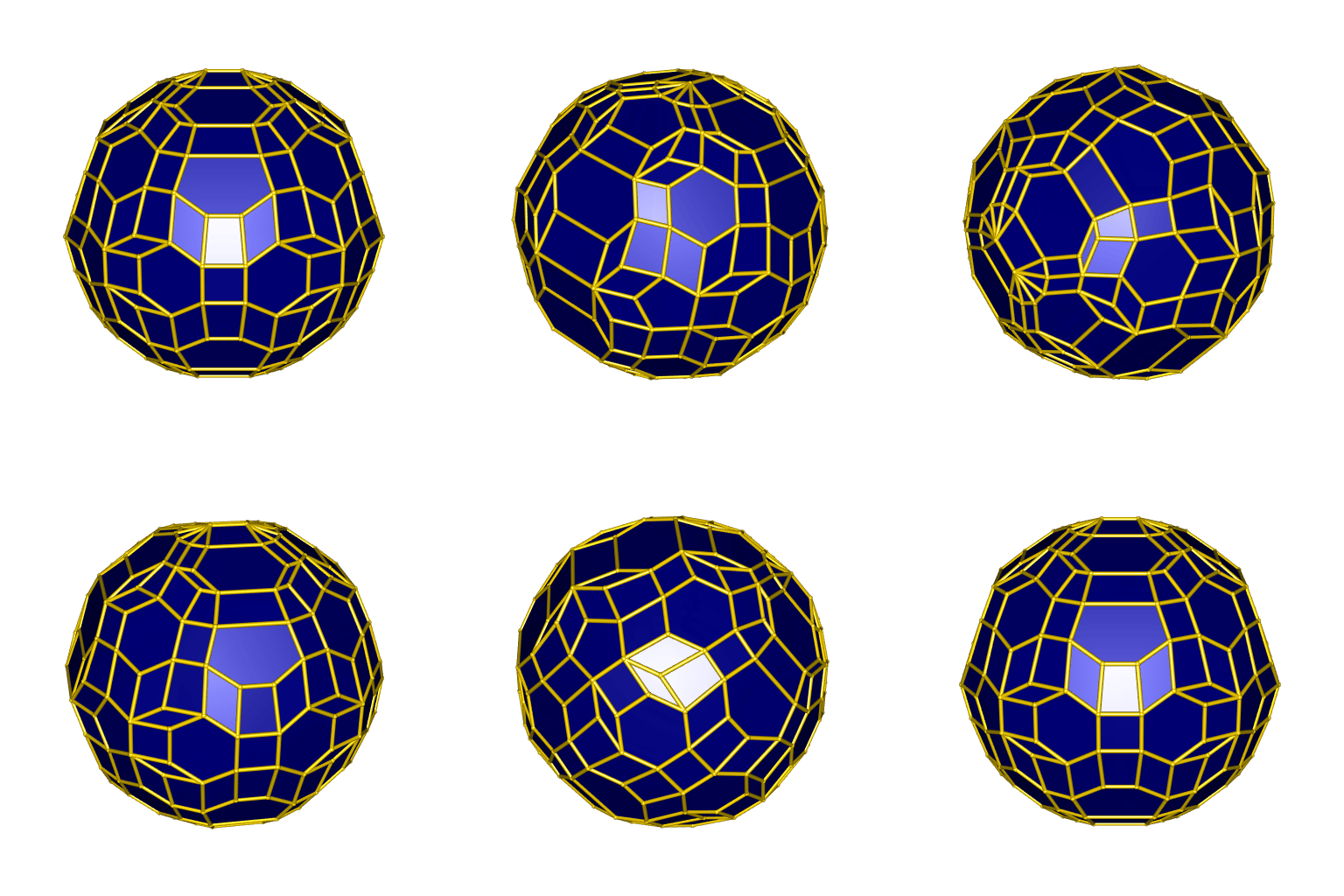
Now let’s see the Minkowski sum of these two polyhedra:

MinkMesh <- MinkowskiSum(Leonardo, truncatedIcosahedron) 

open3d(windowRect = c(50, 50, 562, 562), zoom = 0.8)
shade3d(toRGL(MinkMesh), color="navy")
plotEdges(
  MinkMesh[["vertices"]], MinkMesh[["exteriorEdges"]], 
  color = "gold", tubesRadius = 0.06, spheresRadius = 0.08
)

Beautiful. The generation of the Minkowski sum is fast for this example. But it can be very slow for meshes with numerous vertices.