Heatmap formatting of a table with 'DT'

Posted on April 8, 2023 by Stéphane Laurent

Tags: R, datatables

Googling “heatmap format excel” returns a lot of results. Here we will see how to do a heatmap formatting with a DT table in R.

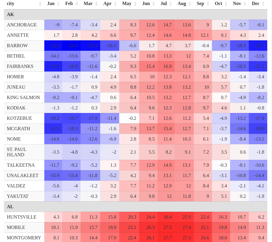
The dataset we use provides the average monthly temperatures over a year for some cities in USA. It is available in a CSV file here.

The table is in long format. Below we turn it into a table in wide format. We also convert the temperatures to Celsius degrees and we rename the months which are given as numbers in the original data.

# read the CSV data
dat0 <- read.csv("TempCitiesUSA.csv")
# it is in long format:
head(dat0)
##   state      city month temp.f
## 1    AK ANCHORAGE     1   15.8
## 2    AK ANCHORAGE     2   18.7
## 3    AK ANCHORAGE     3   25.9
## 4    AK ANCHORAGE     4   36.3
## 5    AK ANCHORAGE     5   46.9
## 6    AK ANCHORAGE     6   54.7
# I prefer Celsius degrees
dat0[["temp.f"]] <- round((dat0[["temp.f"]] - 32) / 1.8, digits = 1L) 
# convert to wide format
library(tidyr)
dat <- dat0 %>% 
  pivot_wider(
    names_from  = month,
    values_from = temp.f
)
# replace the month numbers in the column names
colnames(dat)[3:14] <- month.abb
# have a look
pillar::glimpse(dat, width = 65)
## Rows: 261
## Columns: 14
## $ state <chr> "AK", "AK", "AK", "AK", "AK", "AK", "AK", "AK", "…
## $ city  <chr> "ANCHORAGE", "ANNETTE", "BARROW", "BETHEL", "FAIR…
## $ Jan   <dbl> -9.0, 1.7, -25.4, -14.1, -23.2, -4.8, -3.5, -9.2,…
## $ Feb   <dbl> -7.4, 2.8, -26.6, -13.6, -19.9, -3.9, -1.7, -9.1,…
## $ Mar   <dbl> -3.4, 4.2, -25.4, -9.7, -11.6, -1.4, 0.9, -4.7, 0…
## $ Apr   <dbl> 2.4, 6.6, -18.1, -3.4, -0.2, 2.4, 4.9, 0.6, 2.9, …
## $ May   <dbl> 8.3, 9.7, -6.6, 5.2, 9.3, 6.5, 8.8, 6.4, 6.4, -0.…
## $ Jun   <dbl> 12.6, 12.4, 1.7, 10.8, 15.4, 10.0, 12.2, 10.5, 9.…
## $ Jul   <dbl> 14.7, 14.6, 4.7, 13.3, 16.9, 12.3, 13.8, 13.2, 12…
## $ Aug   <dbl> 13.6, 14.8, 3.7, 12.0, 13.4, 12.1, 13.2, 12.7, 12…
## $ Sep   <dbl> 9.0, 12.1, -0.4, 7.4, 6.9, 8.8, 10.0, 8.7, 9.7, 5…
## $ Oct   <dbl> 1.2, 8.1, -9.7, -1.1, -4.7, 3.2, 5.7, 0.7, 4.6, -…
## $ Nov   <dbl> -5.7, 4.3, -18.3, -8.1, -16.5, -1.4, 0.7, -4.9, 1…
## $ Dec   <dbl> -8.1, 2.4, -23.7, -12.6, -21.1, -3.4, -1.8, -8.2,…

We will use the lowest temperature and the highest temperature later.

# get the lowest and highest temperatures
lowest  <- min(dat0[["temp.f"]])
highest <- max(dat0[["temp.f"]])

Now let’s detail our manipulation for one column. We map the temperatures to the interval \((0,1)\), in such a way that \(0\) is sent to \(0.5\).

# let's detail for one column, January
x <- dat[["Jan"]]
# function to map from (lowest, highest) to (0, 1), mapping 0 to 0.5
interpfun <- splinefun(
  c(lowest, 0, highest),
  c(0, 0.5, 1)
)
# map the January data
y <- interpfun(x)

Now we map each value of y to a color, such that \(0.5\) is sent to white.

# function mapping (0, 1) to a color; 0.5 is sent to white 
colfunc <- colorRamp(c("blue", "white", "red"))
# get the colors for January
cols <- colfunc(y)
# these are rgb codes, we convert them to hex codes
clrs <- rgb(cols[, 1L], cols[, 2L], cols[, 3L], maxColorValue = 255)

In this way the negative temperatures will be colored in blue and the positive temperatures in red.

Now we apply this manipulation for each month.

# now we perform this stuff for each month
Colors <- lapply(dat[, month.abb], function(x) {
  y <- interpfun(x)
  cols <- colfunc(y)
  rgb(cols[, 1L], cols[, 2L], cols[, 3L], maxColorValue = 255)
})
# have a look
str(Colors)
## List of 12
##  $ Jan: chr [1:261] "#AEAEFF" "#FFF0F0" "#0C0CFF" "#7E7EFF" ...
##  $ Feb: chr [1:261] "#BDBDFF" "#FFE7E7" "#0000FF" "#8282FF" ...
##  $ Mar: chr [1:261] "#E1E1FF" "#FFDBDB" "#0C0CFF" "#A7A7FF" ...
##  $ Apr: chr [1:261] "#FFEAEA" "#FFC7C7" "#5757FF" "#E1E1FF" ...
##  $ May: chr [1:261] "#FFB9B9" "#FFAEAE" "#C4C4FF" "#FFD3D3" ...
##  $ Jun: chr [1:261] "#FF9797" "#FF9999" "#FFF0F0" "#FFA5A5" ...
##  $ Jul: chr [1:261] "#FF8787" "#FF8888" "#FFD7D7" "#FF9292" ...
##  $ Aug: chr [1:261] "#FF9090" "#FF8787" "#FFDFDF" "#FF9C9C" ...
##  $ Sep: chr [1:261] "#FFB4B4" "#FF9B9B" "#FBFBFF" "#FFC1C1" ...
##  $ Oct: chr [1:261] "#FFF4F4" "#FFBBBB" "#A7A7FF" "#F5F5FF" ...
##  $ Nov: chr [1:261] "#CCCCFF" "#FFDADA" "#5555FF" "#B6B6FF" ...
##  $ Dec: chr [1:261] "#B6B6FF" "#FFEAEA" "#1E1EFF" "#8C8CFF" ...

Now let’s do the DT table. I use the RowGroup extension to group the data by state (the 0-th column in JavaScript).

library(DT)
dtable <- datatable(
  dat, rownames = FALSE, extensions = "RowGroup", 
  options = list(
    rowGroup = list(dataSrc = list(0)),
    columnDefs = list( # hide the grouping column
      list(targets = 0, visible = FALSE)
    )
  )
)

And now we format this table.

for(month in month.abb) {
  dtable <- dtable %>%
    formatStyle(
      month, 
      backgroundColor = styleEqual(dat[[month]], Colors[[month]])
    )
}

That’s done.

dtable