Two-sided tolerance factor for linear regression

Posted on July 23, 2017 by Stéphane Laurent

We denote by \(\chi^2_{\nu, \lambda}(p)\) the \(100p\%\)-quantile of the non-central Chi-squared distribution \(\chi^2_{\nu, \lambda}\) with degrees of freedom number \(\nu\) and non-centrality parameter \(\lambda\).

As shown in Krishnamoorthy & Mathew’s book, the two-sided \((p, 1-\alpha)\)-tolerance factor for a linear regression model is the solution \(k\) of the equation

\[ \frac{2}{d}\int_0^\infty \Pr\left(\chi^2_\ell > \frac{\ell\chi^2_{1,x^2}(p)}{k^2} \right) \phi\left(\frac{x}{d}\right) \mathrm{d}x = 1-\alpha \] where \(\ell\) is the corank of the \(X\) matrix, and \(d\) is a number calculated from the desired values of the predictors (as we will see on the example).

Below we provide a Rcpp implementation of the integral. We use the boost library (offered by the BH package) to evaluate the integrand, and the package RcppNumerical to evaluate the integral, after transforming this integral to an integral on \((0,1)\).

// [[Rcpp::depends(BH)]]
// [[Rcpp::depends(RcppEigen)]]
// [[Rcpp::depends(RcppNumerical)]]
#include <RcppNumerical.h>
using namespace Numer;
#include <Rcpp.h>
using namespace Rcpp;
#include <boost/math/distributions/non_central_chi_squared.hpp>
#include <boost/math/distributions/complement.hpp>
#include <boost/math/distributions/normal.hpp>
#include <boost/math/distributions/chi_squared.hpp>

// [[Rcpp::export]]
double integrand(double u, double l, double p, double k, double d){
  double x = u/(1-u);
  double q = boost::math::quantile(boost::math::non_central_chi_squared(1, x*x), p);
  double pchisq = boost::math::cdf(boost::math::complement(boost::math::chi_squared(l), l*q/k/k));
  double w = 2*boost::math::pdf(boost::math::normal(0, d), x);
  return w * pchisq / ((1-u)*(1-u));
}

class Integrand: public Func
{
private:
  double l;
  double p;
  double k;
  double d;
public:
  Integrand(double l_, double p_, double k_, double d_) : l(l_), p(p_), k(k_), d(d_) {}
  
  double operator()(const double& u) const
  {
    return integrand(u, l, p, k, d);
  }
};

// [[Rcpp::export]]
Rcpp::NumericVector integral(double l, double p, double k, double d){
  Integrand f(l, p, k, d);
  double err_est;
  int err_code;
  const double res = integrate(f, 0, 1, err_est, err_code);
  Rcpp::NumericVector out = Rcpp::NumericVector::create(res);
  out.attr("err_est") = err_est;
  out.attr("err_code") = err_code;
  return out;
}

Example

We test our function on Example 3.1 of Krishnamoorthy & Mathew’s book. We firstly calculate the value of \(d\).

dat <- data.frame(
  x1 = c(80, 93, 100, 82, 90, 99, 81, 96, 94, 93, 97, 95, 100, 85, 86, 87), 
  x2 = c(8, 9, 10, 12, 11, 8, 8, 10, 12, 11, 13, 11, 8, 12, 9, 12), 
  y = c(2256, 2340, 2426, 2293, 2330, 2368, 2250, 2409, 2364, 2379, 2440, 2364, 2404, 2317, 2309, 2328)
)
fit <- lm(y ~ x1+x2, data=dat)
X <- model.matrix(fit)
H <- chol2inv(chol(t(X)%*%X)) # inverse of X'X
## we want the tolerance interval at x1=88 and x2=9
xnew <- c(1, 88, 9)
d <- sqrt(c(t(xnew) %*% H %*% matrix(xnew)))

No we solve the equation. The Rcpp function integral is available in a package I called regtolerance.

f <- function(k, l, p, d, alpha){
  regtolerance:::integral(l, p, k, d) - (1-alpha)
}
## Calculation of the (0.9, 0.95)-tolerance factor
( k <- uniroot(f, l=nrow(dat)-3, p=0.9, d=d, alpha=0.05, lower=2, upper=3)$root )
## [1] 2.602851

Now we get the tolerance interval as follows:

estimates <- fit$coefficients
yhat <- c(t(xnew) %*% matrix(estimates))
yhat + c(-1,1)*k*sigma(fit)
## [1] 2271.436 2356.594

Bounding the tolerance factor

Lower bound

For a fixed number of degrees of freedom, the Chi-squared distribution is stochastically increasing in its non-centrality parameter. Therefore \[ \frac{2}{d}\int_0^\infty \Pr\left(\chi^2_\ell > \frac{\ell\chi^2_{1,x^2}(p)}{k^2} \right) \phi\left(\frac{x}{d}\right) \mathrm{d}x \leq \Pr\left(\chi^2_\ell > \frac{\ell\chi^2_{1}(p)}{k^2} \right) \]

Thus, the value of \(k\) satisfying \[ \Pr\left(\chi^2_\ell > \frac{\ell\chi^2_{1}(p)}{k^2} \right) = 1-\alpha \] is lower than the tolerance factor.

l <- nrow(dat)-3
p <- 0.9
alpha <- 0.05
# lower bound
sqrt(l*qchisq(p,1)/qchisq(1-alpha, l, lower.tail=FALSE))
## [1] 2.443276

curve(Vectorize(regtolerance:::integral)(l, p, x, d), 
      from=0.1, to=4, ylim=c(0,1))
curve(pchisq(l*qchisq(p,1)/x^2, l, lower.tail=FALSE), add=TRUE, col="red")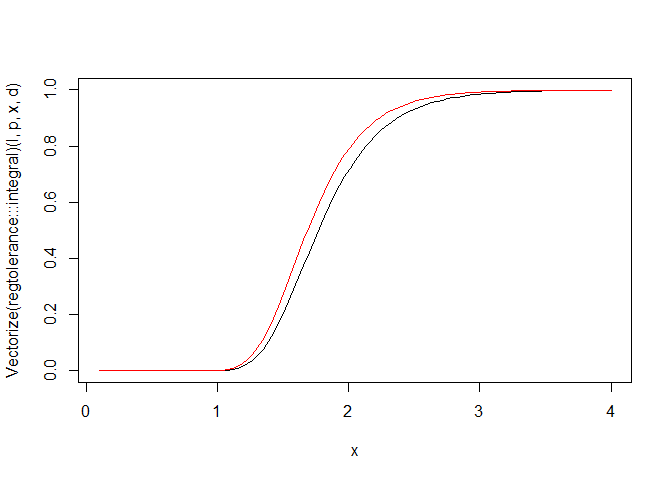

Upper bound

The Lee & Mathew approximation of \(k\) is known to be generally higher than \(k\). It is returned by the function kLM below.

kLM <- function(p, alpha, l, d){
  e <- (1+d^2)^2/d^4
  f <- d^4/(1+d^2) 
  delta <- d^2*((3*d^2+sqrt(9*d^4+6*d^2+3))/(2*d^2+1))
  sqrt(e*f/(1+delta)*qchisq(p, 1, delta)*qf(1-alpha, e, l))
}
kLM(p, alpha, l, d)
## [1] 2.606926

Put things together

p = 0.9 
alpha = 0.05
xnew = c(1, 88, 9)
X <- model.matrix(fit)
H <- chol2inv(chol(t(X)%*%X)) 
d <- sqrt(c(t(xnew) %*% H %*% matrix(xnew)))
l <- nrow(X)-ncol(X)
k_low <- sqrt(l*qchisq(p,1)/qchisq(alpha, l))
k_upp <- kLM(p, alpha, l, d)
( k <- uniroot(f, l = l, p = p, d = d, alpha = alpha, 
               lower = k_low, upper = k_upp, 
               extendInt = "upX")$root )
## [1] 2.602831

References

Krishnamoorthy & Mathew (2009). Statistical Tolerance Regions. Wiley.