Animating a 'rgl' mesh at constant speed

Posted on February 27, 2023 by Stéphane Laurent

Tags: R, graphics, maths, rgl

The purpose of my package qsplines is to construct quaternions splines. This is a port of the Python library splines, written by Matthias Geier. A quaternions spline is a sequence of quaternions interpolating some given quaternions.

One feature I particularly like is the possibility to get a quaternions spline having constant speed. I’m going to illustrate this feature.

Firstly, I take some key points following a spherical curve on the unit ball. Then I will take, for each key point, a unit quaternion (“rotor”) which sends the first key point to this key point, through the rotation it corresponds to. The spherical curve I take is a so-called satellite curve.

# satellite curve
# https://mathcurve.com/courbes3d.gb/satellite/satellite.shtml
satellite <- function(t, R = 1, alpha = pi/2, k = 8) {
  c(
    cos(alpha) * cos(t) * cos(k*t) - sin(t) * sin(k*t),
    cos(alpha) * sin(t) * cos(k*t) + cos(t) * sin(k*t),
    sin(alpha) * cos(k*t)
  )
}
# take key points running on the satellite curve
nkeypoints <- 10L
t_ <- seq(0, 2*pi, length.out = nkeypoints+1L)[1L:nkeypoints]
keyPoints <- t(vapply(t_, satellite, numeric(3L)))

Now the rotors as previously described:

# construction of the key rotors; the first key rotor 
#   is the identity quaternion and rotor i sends the 
#   first key point to the i-th key point
keyRotors <- quaternion(length.out = nkeypoints)
rotor <- keyRotors[1L] <- H1
for(i in seq_len(nkeypoints - 1L)){
  keyRotors[i+1L] <- rotor <-
    quaternionFromTo(keyPoints[i, ], keyPoints[i+1L, ]) * rotor
}

And now the constant speed quaternions spline:

# Kochanek-Bartels quaternions spline interpolating the key rotors
rotors <- KochanekBartels(
  keyRotors, n_intertimes = 10L, 
  endcondition = "closed", tcb = c(0, 0, 0), 
  constantSpeed = TRUE
)

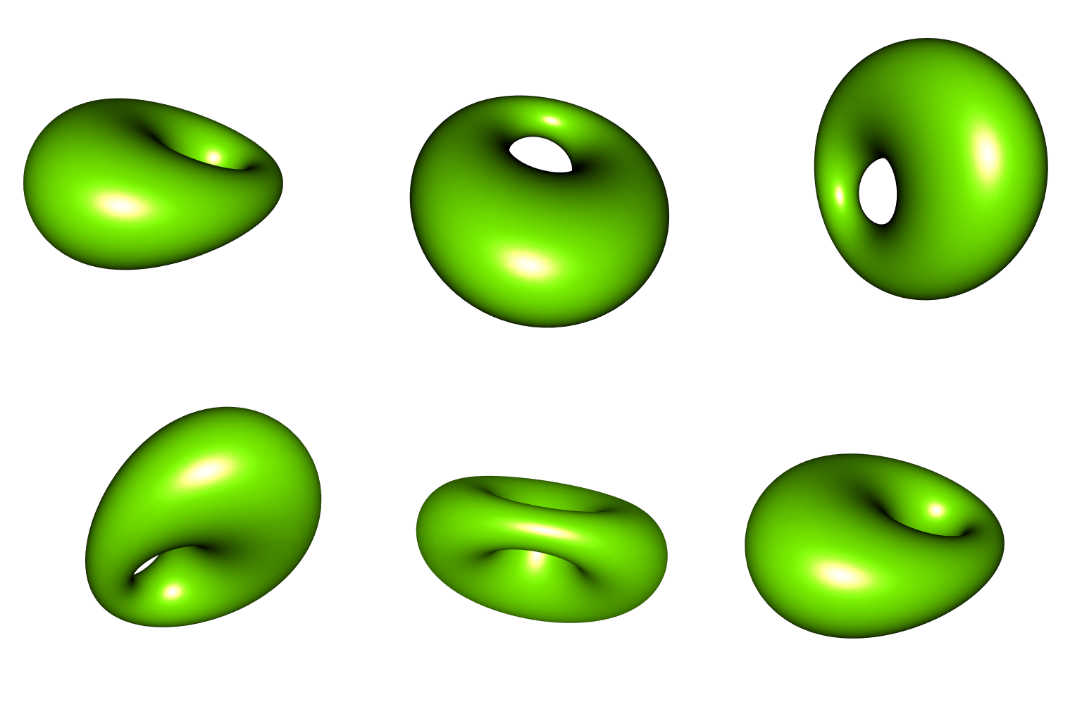
And now, with the help of this spline, we can construct an animation of a rgl mesh rotating at constant speed. I take a mesh of a Dupin cyclide.

library(rgl)
mesh0 <- cgalMeshes::cyclideMesh(
  a = 97, c = 32, mu = 57, nu = 200L, nv = 200L
)
open3d(windowRect = 50 + c(0, 0, 512, 512), zoom = 0.6)
for(i in 1L:length(rotors)) {
  rotMatrix <- as.orthogonal(rotors[i])
  mesh <- rotate3d(mesh0, matrix = rotMatrix)
  # this invisible sphere is used to fix the frame 
  spheres3d(x = 0, y = 0, z = 0, radius = 200, alpha = 0)
  shade3d(mesh0, color = "chartreuse")
  png <- sprintf("pic%03d.png", i)
  snapshot3d(png, webshot = FALSE)
  clear3d()
}
# mount animation
pngFiles <- Sys.glob("*.png")
library(gifski)
gifski(
  pngFiles, "cyclide_constantSpeed.gif",
  width = 512, height = 512,
  delay = 1/10
)
file.remove(pngFiles)

If you want to play with this stuff, you can change the parameters of the satellite curve to get a different motion, and also change the tcb argument in the KochanekBartels function (tension, continuity, bias). There is a Shiny application in qsplines allowing to visualize the effects of tcb.