Why I like generalized fiducial inference

Posted on November 8, 2020 by Stéphane Laurent

Tags: R, maths, statistics

Throughout this article, one considers the balanced one-way ANOVA model with a random factor (group). The between standard deviation and the within standard deviation are denoted by \(\sigma_{\mathrm{b}}\) and \(\sigma_{\mathrm{w}}\) respectively. The grand mean is denoted by \(\mu\). The number of levels of the group factor is denoted by \(I\) and the number of individuals within each group is denoted by \(J\). Thus the model is: \[ \mu_i \sim_{\text{iid}} \mathcal{N}(\mu, \sigma_{\mathrm{b}}^2), \, i = 1, \ldots, I \qquad (y_{i,j} \mid \mu_i) \sim_{\text{iid}} \mathcal{N}(\mu_i, \sigma_{\mathrm{w}}^2), \, j = 1, \ldots, J. \]

Using ‘rstanarm’ with the default priors

Below I fit the model with the ‘rstanarm’ package for fifteen simulated datasets with \(I = 10\), \(J = 5\), \(\mu = 10000\), \(\sigma_{\mathrm{b}} = 50\), \(\sigma_{\mathrm{w}} = 1\). I assign a “vague” half-Cauchy prior distribution to \(\sigma_{\mathrm{w}}\) and the other prior distributions are the default prior distributions of stan_lmer.

library(rstanarm)
options(mc.cores = parallel::detectCores())

mu           <- 10000 
sigmaWithin  <- 1
ratio        <- 50
sigmaBetween <- sigmaWithin * ratio
I            <- 10L 
J            <- 5L 

nsims <- 15L 

stanIntervals <- list( # to store the confidence intervals
  within = `colnames<-`(matrix(NA_real_, nrow = nsims, ncol = 3), 
                      c("estimate", "lwr", "upr")),
  between = `colnames<-`(matrix(NA_real_, nrow = nsims, ncol = 3), 
                      c("estimate", "lwr", "upr"))
)

set.seed(666L)

for(i in 1L:nsims){
  groupMeans <- rnorm(I, mu, sigmaBetween)
  y          <- c(
    vapply(groupMeans, function(gmean) rnorm(J, gmean, sigmaWithin), numeric(J))
  )
  dat        <- data.frame(
    y = y,
    group = gl(I, J)
  )
  
  rstanarm <- stan_lmer(
    y ~ (1|group), data = dat, iter = 5000L,
    prior_aux = cauchy(0, 5)
  )
  
  pstrr <- as.data.frame( # extract posterior draws
    stan,
    pars = c(
      "(Intercept)",
      "sigma",
      "Sigma[group:(Intercept),(Intercept)]"
    )
  )
  names(pstrr)[2L:3L] <- c("sigma_error", "sigma_group")
  pstrr[["sigma_group"]] <- sqrt(pstrr[["sigma_group"]])

  x <- t(vapply(pstrr, quantile, numeric(3L), probs = c(50, 2.5, 97.5)/100))
  stanIntervals$within[i, ] <- x["sigma_error", ]
  stanIntervals$between[i, ] <- x["sigma_group", ]
}

Let’s plot the intervals now.

library(ggplot2)
stanWithin <- as.data.frame(stanIntervals[["within"]])
stanWithin[["simulation"]] <- factor(1L:nsims)
ggplot(
  stanWithin, 
  aes(
    x = simulation, y = estimate, ymin = lwr, ymax = upr
  )
) + 
  geom_pointrange() + 
  ylab("interval") + 
  geom_hline(yintercept = 1, linetype = "dashed") + 
  ggtitle("Confidence intervals about the within standard deviation")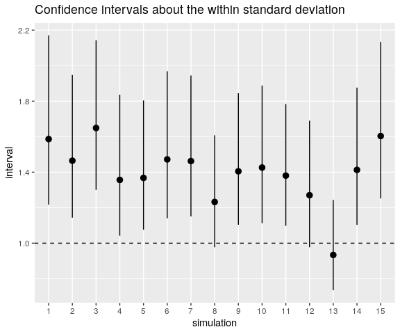

The horizontal line shows the value of \(\sigma_{\mathrm{w}}\). As you can see, the confidence intervals dramatically fail to catch this value.

And this is also the case for \(\sigma_{\mathrm{b}}\):

stanBetween <- as.data.frame(stanIntervals[["between"]])
stanBetween[["simulation"]] <- factor(1L:nsims)
ggplot(
  stanBetween, 
  aes(
    x = simulation, y = estimate, ymin = lwr, ymax = upr
  )
) + 
  geom_pointrange() + 
  ylab("interval") + 
  geom_hline(yintercept = 1, linetype = "dashed") + 
  ggtitle("Confidence intervals about the between standard deviation")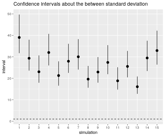

Resolving the issue

Why? The explanation is simple: stan_lmer assigns a unit exponential prior distribution to the between standard deviation, which is equal to \(50\).

So we have to change this prior distribution, and stan_lmer allows to use a Gamma distribution as the prior distribution of the between standard deviation. Its parameters shape and scale are settable in the decov function which is passed on to the prior_covariance option:

rstanarm <- stan_lmer(
  y ~ (1|group), data = dat, iter = 5000L,
  prior_aux = cauchy(0, 5),
  prior_covariance = decov(shape = 2, scale = 30)
)

I choose the \(\textrm{Gamma}(\textrm{shape}=2, \textrm{scale=30})\) distribution because it has median \(\approx 50\) and is “vague” enough: its equi-tailed \(95\%\)-dispersion interval is \(\approx (7, 167)\).

☛ However it took me some time to pick up these parameters. I firstly tried a more dispersed Gamma distribution but stan_lmer returned a bunch of warnings and non-sensible results.

Below are the confidence intervals obtained with this Gamma prior distribution. I compare them with the frequentist intervals obtained with the ‘AOV1R’ package.

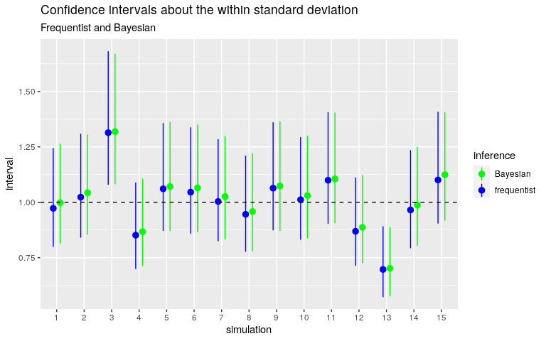
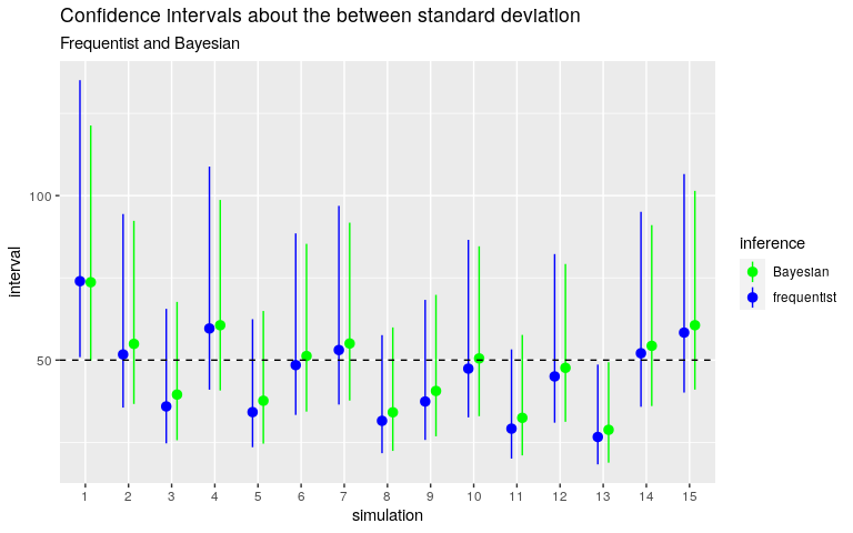
Quite good.

☛ I also noticed that the sampling was slower with this Gamma distribution.

Try the generalized fiducial inference.

My new package ‘gfilmm’ allows to perform the generalized fiducial inference for any Gaussian linear mixed model with categorical random effects.

Fiducial inference and Bayesian inference have something in common: they are both based on a distribution representing the uncertainty about the parameters: the fiducial distribution and the posterior distribution, respectively.

A notable difference between these two methods of inference is that there’s no prior distribution in fiducial statistics.

Here is how to run the fiducial sampler:

library(gfilmm)
fiducialSimulations <- gfilmm(
  y = ~ cbind(y - 0.01, y + 0.01), fixed = ~ 1, random = ~ group, 
  data= dat, N = 10000L
)

Note the form of the response variable: ~ cbind(y - 0.01, y + 0.01). That’s because the generalized fiducial inference applies to interval data.

Below are the fiducial confidence intervals for the same simulated datasets as before.

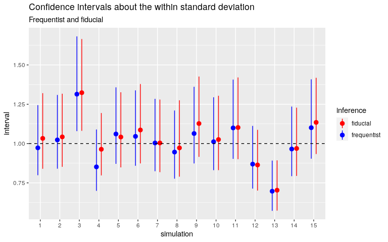
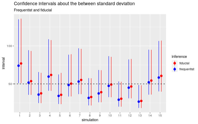
Quite good too. And let me insist on this point: there is no prior distribution, there is nothing to set, except the number of simulations. I implemented the algorithm (due to J. Cisewski and J. Hannig) in C++ and it takes less than 1000 lines of code.

Let’s increase the between standard deviation now.

ratio <- 1000
sigmaBetween <- ratio * sigmaWithin
set.seed(31415926L)
groupMeans <- rnorm(I, mu, sigmaBetween)
y          <- c(
  vapply(groupMeans, function(gmean) rnorm(J, gmean, sigmaWithin), numeric(J))
)
dat        <- data.frame(
  y = y,
  group = gl(I, J)
)
library(AOV1R)
library(gfilmm)
aovfit <- aov1r(y ~ group, data = dat)
gf <- gfilmm(~ cbind(y-0.01, y+0.01), ~ 1, ~ group, data = dat, N = 5000L)
confint(aovfit)
##               estimate          lwr          upr
## grandMean 9783.4770335 9227.6673527 10339.286714
## within       0.9454425    0.7762205     1.209696
## between    776.9682432  534.4260219  1418.441282
## total      776.9688185  534.4268604  1418.441598
## 
## attr(,"confidence level")
## [1] 0.95
## attr(,"standard deviations")
## [1] TRUE

gfiSummary(gf)
##                    mean      median         lwr          upr Pr(=0)
## (Intercept) 9786.579629 9787.161625 9247.718851 10344.743737     NA
## sigma_group  854.314055  807.650667  528.463101  1485.287694      0
## sigma_error    1.557918    1.543563    1.273913     1.931306      0
## attr(,"confidence level")
## [1] 0.95

The fiducial confidence interval about the within standard deviation does not match the frequentist interval, and does not catch the true value. Nothing to tinker with, except the number of simulations:

gf <- gfilmm(~ cbind(y-0.01, y+0.01), ~ 1, ~ group, data = dat, N = 30000L)
gfiSummary(gf)
##                     mean       median          lwr          upr Pr(=0)
## (Intercept) 9780.0741293 9779.1304187 9230.1017080 10333.801655     NA
## sigma_group  847.3551078  805.8588214  536.0212551  1401.862597      0
## sigma_error    0.9540852    0.9455375    0.7762872     1.185648      0
## attr(,"confidence level")
## [1] 0.95

Now the fiducial intervals match the frequentist ones.

Epilogue

As you have seen, using the generalized fiducial inference is easy, easier than the Bayesian inference. The difficulty I mentioned regarding the Bayesian inference is not severe, but this is because the one-way ANOVA model with a random factor is the simplest Gaussian linear mixed model. Namely, it has only one between standard deviation. Things get more complicated for a mixed model with multiple random effects. With rstanarm::stan_lmer, one has to assign a Gamma prior distribution on each between standard deviation. I cheated for the above example: I did multiple attempts to select the parameters of the Gamma prior, until I found results close to the frequentist ones!