The Mandelbulb in R

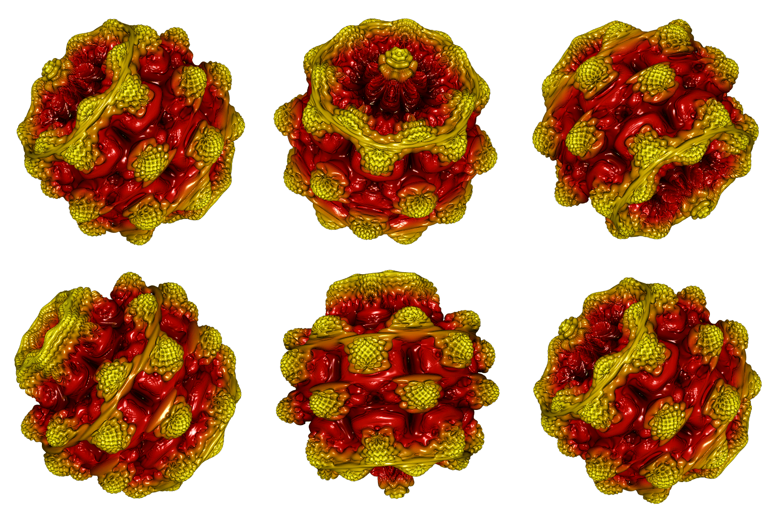
Posted on February 8, 2023 by Stéphane Laurent

Tags: R, Rcpp, rgl

In this post, I provide some R code which generates a mesh of the Mandelbulb, a well-known 3D fractal.

The Mandelbulb is an isosurface, and I use the rmarchingcubes package to get a mesh of this isosurface. Since the Mandelbulb has many details, a thin grid of the voxel space is necessary, and that is why I use Rcpp to generate the voxel. Here is the C++ code:

// file mandelbulb.cpp
#include <Rcpp.h>
using namespace Rcpp;

double mandelbulb0(
  double x, double y, double z, const unsigned power, const double phase
) {
  const double x0 = x;
  const double y0 = y;
  const double z0 = z;
  const double k = power;
  double r, rkm1, rk, theta, phi;
  double dr = 1.0;
  int i;
  for(i = 0; i < 10; i++) {
    r = sqrt(x*x + y*y + z*z);
    if(r > 2) {
      return 2.0 * r * log(r) / dr;
    }
    rkm1 = pow(r, k - 1.0);
    dr = k * rkm1 * dr + 1.0;
    theta = k * atan2(sqrt(x*x + y*y), z) + phase;
    phi   = k * atan2(y, x);
    rk = rkm1 * r;
    x = rk * cos(phi) * sin(theta) + x0;
    y = rk * sin(phi) * sin(theta) + y0;
    z = rk * cos(theta) + z0;
  }
  return 0.0;
}

// [[Rcpp::export]]
NumericVector mandelbulb(
  const double m, const double M, const unsigned n, 
  const unsigned power, const double phase
) {
  NumericVector out(n * n * n);
  const double h = (M - m) / (n - 1);
  double x, y, z;
  unsigned i, j, k;
  unsigned l = 0;
  for(i = 0; i < n; i++) {
    x = m + i*h;
    for(j = 0; j < n; j++) {
      y = m + j*h;
      for(k = 0; k < n; k++) {
        z = m + k*h;
        out(l) = mandelbulb0(x, y, z, power, phase);
        l++;
      }
    }
  }
  out.attr("dim") = Dimension(n, n, n);
  return out;
}

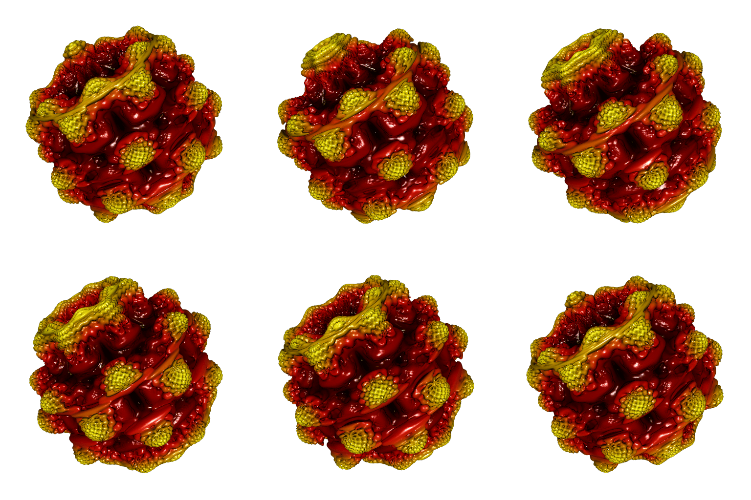
In fact, there are several Mandelbulb, each corresponding to a value of the power argument in the above code. The most popular one is the one with power=8. At the end of this post, I’ll show you the effect of the phase argument.

Now here is the R code which generates the mesh:

Rcpp::sourceCpp("mandelbulb.cpp")

library(rmarchingcubes)
library(rgl)

n <- 512L # more than enough
x <- y <- z <- seq(-1.2, 1.2, length.out = n)

voxel <- mandelbulb(-1.2, 1.2, n, 8L, 0)
ctr   <- contour3d(voxel, level = 0.01, x = x, y = y, z = z)

mesh <- tmesh3d(
  vertices = t(ctr[["vertices"]]),
  indices  = t(ctr[["triangles"]]),
  normals  = ctr[["normals"]],
  homogeneous = FALSE
)

This mesh can be plotted with rgl. But let’s add some color before. I like the ‘klingon’ color palette of the trekcolors package.

library(trekcolors)
fpalette <- colorRamp(trek_pal("klingon", reverse = TRUE))
d2 <- apply(mesh[["vb"]][-4L, ], 2L, crossprod)
d2 <- (d2 - min(d2)) / diff(range(d2))
RGB <- fpalette(d2)
mesh[["material"]] <- list(
  "color" = rgb(RGB[, 1L], RGB[, 2L], RGB[, 3L], maxColorValue = 255)
)

open3d(windowRect = c(50, 50, 562, 562), zoom = 0.7)
shade3d(mesh, shininess = 128)

The animation below shows the effect of the phase argument, varying from \(0\) to \(2\pi\):