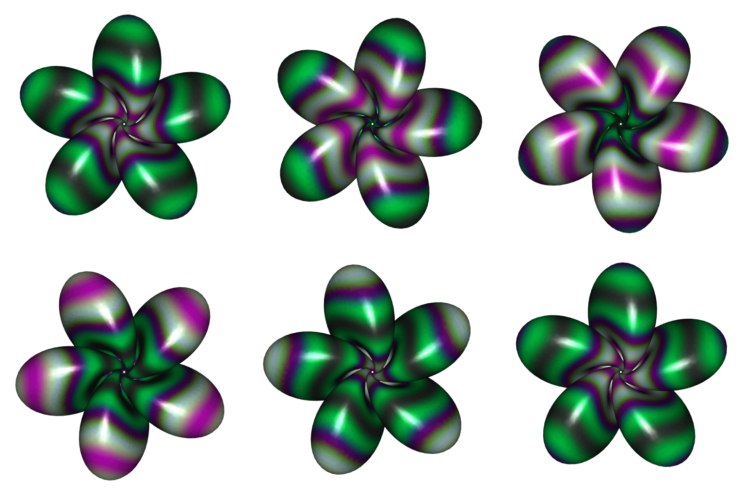
Hopf torus with dynamic colors

In a recent post I explained how to decorate a surface with moving colors with the Python library PyVista. Here I expose this method for the R package rgl.

I will take a Hopf torus with fives lobes for the illustration. The following R function is a slight modification of the parametric3d function of the misc3d package. It is more efficient for the Hopf torus parameterization and it returns a rgl object of class mesh3d.

library(misc3d)
library(rgl)

parametricMesh3d <- function(
  Fxyz, umin, umax, vmin, vmax, nu, nv 
){
  u <- seq(umin, umax, length.out = nu)
  v <- seq(vmin, vmax, length.out = nv)
  tg <- misc3d:::expandTriangleGrid(u, v)
  f <- function(uv) Fxyz(uv[, 1L], uv[, 2L])
  v1 <- f(tg$v1)
  v2 <- f(tg$v2)
  v3 <- f(tg$v3)
  tris <- makeTriangles(v1, v2, v3)
  mesh0 <- misc3d:::t2ve(tris)
  addNormals(
    tmesh3d(
      vertices = mesh0$vb,
      indices  = mesh0$ib
    )
  )
}

The R function below is the parameterization of the Hopf torus.

HTxyz <- function(u, v, nlobes = 5, A = 0.38){
  C <- pi/2 - (pi/2-A)*cos(u*nlobes)
  sinC <- sin(C)
  D <- u + A*sin(2*u*nlobes)
  p1 <- cos(C) + 1
  p2 <- sinC * cos(D)
  p3 <- sinC * sin(D)
  cos_v <- cos(v)
  sin_v <- sin(v)
  x1 <- cos_v*p3 + sin_v*p2
  x2 <- cos_v*p2 - sin_v*p3
  x3 <- sin_v * p1
  xden <- sqrt(2*p1) - cos_v*p1
  cbind(x1/xden, x2/xden, x3/xden)
}

Let’s make the Hopf torus mesh now.

mesh <- parametricMesh3d(
  HTxyz, umin = 0, umax = 2*pi, vmin = -pi, vmax = pi, nu = 600, nv = 400
)

We will assign a color to each point on the surface, according to the distance from the point to the origin. We calculate these distances below, and we linearly map them to the interval \([0, 2\pi]\).

d <- sqrt(apply(mesh$vb[-4L, ], 2L, crossprod))
d <- 2*pi * (d - min(d)) / diff(range(d))

Now we introduce a color palette function. The trekcolors package has nice color palettes. I’m taking the dominion palette.

library(trekcolors)
fpalette <- colorRamp(
  trek_pal("dominion"), bias = 0.6, interpolate = "spline"
)

This function fpalette assign a color, given by its RGB values, to each number between \(0\) and \(1\). As in Python, we will calculate \(\sin(d -t)\) to move the colors, with \(t\) varying from \(0\) to \(2\pi\). The sine function takes its values in \([-1, 1]\) so we will map this interval to \([0,1]\) with the affine function \(x \mapsto \frac{x+1}{2}\) in order to apply the fpalette function.

We will also rotate the Hopf torus around the \(z\)-axis. By the symmetry of the Hopf torus, it suffices to make the rotation with an angle varying from \(0\) to \(2\pi/5\).

t_ <- seq(0, 2*pi, length.out = 73)[-1L]
angle_ <- seq(0, 2*pi/5, length.out = 73)[-1L]
for(i in seq_along(t_)){
  RGB <- fpalette( (sin(d-t_[i])+1)/2 )
  mesh[["material"]] <- 
    list(color = rgb(RGB[, 1L], RGB[, 2L], RGB[, 3L], maxColorValue = 255))
  rmesh <- rotate3d(mesh, angle_[i], 0, 0, 1)
  open3d(windowRect = c(50, 50, 562, 562))
  view3d(0, 0, zoom = 0.55)
  spheres3d(0, 0, 0, radius = 11, color = "white", alpha = 0) # to fix the view
  shade3d(rmesh)
  rgl.snapshot(sprintf("pic%03d.png", i))
  close3d()
}

This code generates a series of png files pic001.png, …, pic072.png. Using ImageMagick or gifski, we obtain this gif animation from these files:

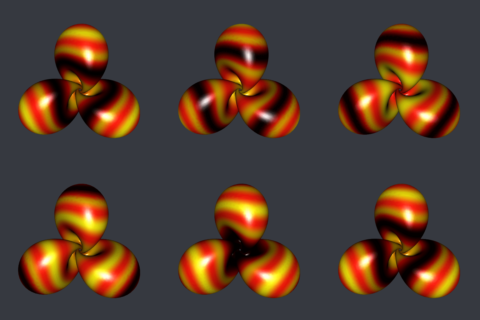
Very well. But these are not my favorite colors. And I prefer the Hopf torus with three lobes. Below it is, decorated with the klingon color palette of trekcolors; I prefer this one.